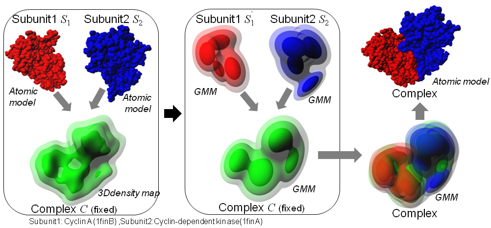
The program gmfit superimposes molecular subunits into the density map of their complex. To reduce computational costs for the superimposiing, both subunits and complexes are transformed into GMM (Gaussian Mixture Model). Transformation of molecular models into GMM can be done usint another program gmconvert. The program is designed to superimpose multiple atomic models of subunits into a low-resolution 3D density map, however, it is also applied to superimposing two 3D density maps, or two atomic models.
The source code of gmfit is written in C assuming the compiler "gcc" in Linux environment. After you download the file "gmfit-src-[date].tar.gz", just type following commands:
tar zxvf gmfit-src-[date].tar.gz
cd src
make
Then you will find the execute file "gmfit" in the upper directory (../src).
We prepare two methods to input parameters for the program gmfit. The first method is using arguments of the command gmfit, the second method is preparing the parameter file for the program. An example of the argument is input a command as follows:
gmfit -cg 1afwAB_r10_g16.gmm -sg1 1afwA_g8.gmm -sg2 1afwB_g8.gmm -sa1 1afwA.pdb -sa2 1afwB.pdb -NI 1000The same calculation can be done using the parameter file method. If you prepare the following file "1afw.gmfit":
  ## <1afw.gmfit> ##
  -cg 1afwAB_r10_g16.gmm
  -sg1 1afwA_g8.gmm
  -sg2 1afwB_g8.gmm
  -sa1 1afwA.pdb
  -sa2 1afwB.pdb
  -NI 1000
Lines starting with '#' are comments, not read by the program. You input just a following command, then the gmfit will start the calculation.
gmfit -script 1afw.gmfitYou can use both argument and a parameter file, such as follows:
gmfit -script 1afw.gmfit -NI 10If the same option (in this case '
-NI') is assigned by both argument and script file, the option value given by the argument has a priority:
'-NI' is set to '10', not '100'.
Details of these options and parameter files will be shown using the option '-h'.
gmfit -h
The system for the gmfit is composed of two types of molecule:COMPLEX and SUBUNIT.
-cg' option.
-cg : input GMM for the complex []The SUBUNIT molecule is one of the element molecule composing the COMPLEX molecule. Their positions and orientations are optimezed by the program. We assume the SUBUNIT molecule is represented by both atomic model and GMM. The file for atomic model of the i-th SUBUNIT is assined by the option '
-sa[i]' (-sa1, -sa2, -sa3,...).
The file for GMM of the i-th SUBUNIT is assined by the option '-sg[i]' (-sg1, -sg2, -sg3,...).
-sa1,-sa2,-sa[x]: input atomic PDB file for 1st,2nd,x-th subunits (MAX_SUBUNIT 21)[  ]
-sg1,-sg2,-sg[x]: input GMM for 1st,2nd,x-th subunits (MAX_SUBUNIT 21)[  ]
The program gmfit searches the optimal configurations of subunits by two steps.
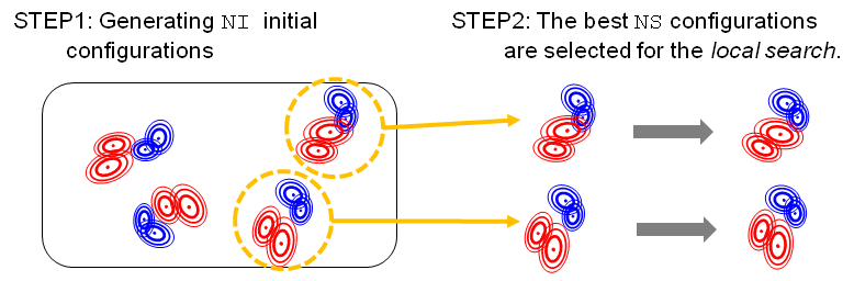
-NI'.
Among NI configuration, only the best NS configurations are optimized by the local search.
Number of locally optimized configurations is assigned by the option '-NS'.
Finally, the best NO configurations are written
Number of output configurations is assigned by the option '-NO'.
-NI  : number of initial configurations. [10]
-NS  : number of configurations for local search [10]
-NO  : number of output configurations [1]
Detals for each step are summarized as follows.
- STEP 1:Generate initial configurations
The method for generating random initial configuraions is assigned by the option '-I', among several different methods.
-I : Initial Configuration. 'R':random, 'P':principal axis fitting, 'Y':symmetric,'F':segment-fitting : 'y:symmetric segment fitting, 'L':local transformation to the original config,'O':keep original config.[R]- 'R':random generation
A center position of each subunit is randomly chosen from the disribution of COMPLEX GMM. A orientation of each subunit is randomly chosen. - 'SF':segmentation fitting
Random configuration is repeatedly improved by the segmentation fitting algorithm. This algorithm can provide much better configuration by the simple random generation method. The detail of the algorithm will be published elsewhere. - 'Y':Symmetric random generation
If the COMPLEX has a rotational symmetry, the symmetric constraint can be used to generate random configurations. To use this option '-I Y', symmetries of subunits should be assigned by '-symunit[x]' and '-symtype[x]'. - 'SFY':segmentation fitting with symmetric constraint
The segmentation fitting algorithm also can provide symmetric configutarions. To use this option '-I SFY', symmetries of subunits should be assigned by '-symunit[x]' and '-symtype[x]'. - 'DG':distance geometry
The distance geometry algorithm effectively generates configurations satisfying the given proximity restraints. The proximity restraints should be assigned by options '-c[x]_[y] 1'. - 'DGSF':distance geometry + segmenration fitting
This is the combination of distance-geoemtry and segmentation fitting algorithms. Initial configurations of the segmentation fitting are generated by the distance geometry. The proximity restraints should be assigned by options '-c[x]_[y] 1'. - 'DGSFY':distance geometry + segmenration fitting with symmetric constraint
This is the combination of distance-geoemtry and segmentation fitting algorithms with symmetric constraints. Initial configurations of the segmentation fitting are generated by the distance geometry. The proximity restraints should be assigned by options '-c[x]_[y] 1'. The symmetry restraints should be assigned by '-symunit[x]' and '-symtype[x]'. - 'P':principal axis fitting
This is for the case with one subunit (Nsubunit=1). A center position of the subunit is set to the center of the complex. If the number-NIis equal to 4, the 4 orientations of the subunit are genrated by matching three principal axis of the subunit with those of the complex by the order of their eigen values. If the number-NIis equal to 24, orientations of the subunit are genrated by matching three principal axis of the subunit with those of the complex without considering the order of their eigen values. If the number-NIis more than 24, the random generation procedure (same as-I R) is performed to generate aditional random initial configurations with the number more than 24. - 'O': use the input original configuration as the initial
The input original configuration of the subunits (assigned by-sg[x]and-sa[x]) is used as the initial configuration. - 'L': Local transformation to the orignal configuration
Random transformations are applied to to the original configuration. Maximum translational vector and rotational angle can be controlled by the options-tviand-rai.-tvi : maximum tranlational vector for random initial configuration (angstrom) [1.000000] -rai : maximum rotational angle for random initial configuration (degree)[10.000000]
- 'R':random generation
- STEP 2:Local search
The method for the local search is assigned by the option
-S.-S : Local search method. 'S'teepest Descent, 'I':keep initial configurations [S]
In the detault setting,the local search will be performed by the steepest descent method.
All the results will be written in the output directory, assigned by the option '-odir'. The default output directory is the current directory (.).
-odir : Output directory for optimizing results [.]In the output directory assigned by
-odir, following files will be written.
- init.sum:summary of iniital configutations.
- gopt.sum:summary of optimized configutations after the local search. This file contains values of various energies,
correlation coefficient between the complex and the subunits, RMSD of subunits from the inital configurations, and so on.
- gopt[rank].gmm: GMM for the [rank]-th best energy configuration
- gopt[rank].pdb: Atomic model for the [rank]-th best energy configuration
-ochimera : output UCSF Chimera command files(*.com) for generating optimal subunit configurations (T or F)[F]If you add the option
-chimera T , the file gopt[rank].com will be written in the output directory.
This file contains translational and rotational operations for the optimal configuration of the subunits for UCSF Chimera.
-KV : Key-Value style stdout ('T' or 'F') [F]
This option is useful to use the gmfit program as a function of shell/interpreter scripts.
If you add the option -KV T , the program output summaries of optimal configuration of the subunits
in the standard output as a simple "key value" style. The first character of the key-value line is not '#',
whereas all of other comment standard output of gmfit program starts with '#'. An example of the key-value style output is as follows:
Etotal_GBEST1      -5.396499e-06
EcmpfitGG_GBEST1   -5.690858e-06
ErepulsGG_GBEST1   2.943599e-07
CorrCoeffGG_GBEST1 0.688556
RMSDorigGG_GBEST1  32.002461
RotMtrx1_Subunit1_GBEST1  -0.337420:0.934130:-0.116396
RotMtrx2_Subunit1_GBEST1  0.532983:0.291497:0.794329
RotMtrx3_Subunit1_GBEST1  0.775936:0.205985:-0.596233
TransVec_Subunit1_GBEST1  85.488688:-101.921700:79.514610
RotMtrx1_Subunit2_GBEST1  -0.593195:-0.378217:-0.710684
RotMtrx2_Subunit2_GBEST1  0.253443:0.750154:-0.610766
RotMtrx3_Subunit2_GBEST1  0.764125:-0.542421:-0.349131
TransVec_Subunit2_GBEST1  99.788266:31.033894:92.659104
-nofout : No File Output ('T' or 'F') [F]
If you add the option -nofout T , the program does not generate any output files, except the standard out.
Symmetrical constrants can be assigned by the options
symtype[x] and symunit[x]:
##options for homo multimer symmetry##
 -symtype[n]: symmetric group type for [n]-th homo multimer group. [n] is 1,2,3,..[]
            : 'C2',...'C7','D2','D3','SC2','SC3',...,'SC7' are acceptable.
 -symunit[n]: subunit id numbers for [n]-th homo multimer group. [n] is 1,2,3,...,[]
            : subunit id numbers  are given by camma-splited-form, such as '1,2,3','2,4,6,8,10'.
For example, if the subunits 1,2,3 are idential, and they have 120-degree rotational symmetry, you should assign "-symtype1 C3 -symunit1 1,2,3".
If the complex is composed of two types of chains (alpha and beta), is composed of three alpha chains (subunit 1,2,3) and
three beta chains (subunits 4,5,6), and these three chains have 120-degree rotational symmetry,
you should assign "-symtype1 C3 -symunit1 1,2,3 -symtype2 C3 -symunit2 4,5,6".
The symmetry types with the "SC" means "self-symmetry":one subunit has the rotational symmetry and the subunit's symmetric axis should align with the symmetric axis of the complex. For example, the option "-symtype1 SC2 -symunit1 1" means that the subunit 1 and the complex have C2 symmetry, their symmetric axis should be aligned.
Please keep in mind that the symmetric constraint only works for subunit-GMMs with the same shape.
The "same" means the very strict sense; the subunit GMMs should contain
the "same" number of the "same"-shape gaussian distribution functions
with the "same" configurations. The pose (orientation and position) of the subunit GMM can be different.
If you do not have a special reason, you would be better assign the same GMM file for subunits under symmetric constraints.
If you use -tpdb option of gmconvert program, you can make the same shape GMM with the different pose
from a homo oligomeric PDB file (see tutorial).
For the first simple calculation, we will show procedures for superimpose two identical subunits into a simulated low resolution map of dimeric complex structure, using PDB entry 1afw. We have to prepare three PDB files, "1afwAB.pdb":the 3D structure for the dimer, "1afwA.pdb" :the 3D structure of the subunit A, "1afwB.pdb" :the 3D structure of the subunit B. These files will be transformed into GMMs using the program gmconvert. The PDB file of the complex is transformed into the simulated low resolution map, and the low resolition map is then converted into GMM with Ngauss = 16.
gmconvert -ipdb 1afwAB.pdb -reso 10.0 -gw 4.0 -omap 1afwAB_r10.map
gmconvert -imap 1afwAB_r10.map -ng 16 -ogmm 1afwAB_r10_g16.gmm
Each atomic model is converted into GMM with Ngauss = 8.
gmconvert -ipdb 1afwA.pdb -ng 8 -ogmm 1afwA_g8.gmm
gmconvert -ipdb 1afwB.pdb -ng 8 -ogmm 1afwB_g8.gmm
Then a following parameter file "1afw.gmfit" is prepared:
  ## <1afw.gmfit> ##
  -cg 1afwAB_r10_g16.gmm
  -sg1 1afwA_g8.gmm
  -sg2 1afwB_g8.gmm
  -sa1 1afwA.pdb
  -sa2 1afwB.pdb
  -odir result_dir
  -I R
  -NI 1000
  -NS 100
  -NO 10
Finally, the following command generates several result files into the directory assigned by '-odir' option.
mkdir result_dir
gmfit -script 1afw.gmfit
The next problem is fitting an atomic model of a complex into a density map of the same complex.
The yeast's ribosome structure is taken for the example.
The atomic model taken from PDB code 3o2z (40S) and 3o58 (60S) is going to be fitted into the density map of EMDB-1067.
You should prepare PDB files "pdb3o2z.ent" and "pdb3o58.ent" and the density map (emdb-1067.map).
These two pdb files are merged into one file "3o2z_3o58.pdb".
cat pdb3o2z.ent pdb3o58.ent > 3o2z_3o58.pdbThis PDB file is converted into GMM with Ngauss = 10.
gmconvert -ipdb 3o2z_3o58.pdb -ng 10 -ogmm 3o2z_3o58_g10.gmmNext, the density map "emdb_1067.map" is converted into GMM with Ngauss = 10. Because the grid size of the map is rather large (125x125x125), we use the option
-rsc 2.
gmconvert -imap emd_1067.map -ng 10 -rsc 2 -ogmm emd_1067_g10.gmmFinally, the program gmfit is executed by the following arguments:
gmfit -cg emd_1067_g10.gmm -sg1 3o2z_3o58_g10.gmm -sa1 3o2z_3o58.pdb -I R -NI 10 -NS 10 -NO 1You will find the fitted PDB file "
gopt1.pdb" in the current directory.
In this tutorial, fitting a density map of E.coli ribosome into another density map of yeast ribosome.
Before the calculation, two data of density maps ("emd_1915.map" and "emd_1915.map") are downloaded from EMDB.
Next, these two density maps are converted into GMM with 10 Gaussian functions. To enhance the computational speed, we limit maximum voxel length to 64.
gmconvert -imap emd_1915.map -ng 10 -maxsize 64 -ogmm emd_1915_g10.gmm
gmconvert -imap emd_1067.map -ng 10 -maxsize 64 -ogmm emd_1067_g10.gmm
The map
emd_1915.map is superimposed into the map emd_1067.map by a following command.
gmfit -cg emd_1067_g10.gmm -sg1 emd_1915_g10.gmm -I P -ochimera TAfter the fitting calculation, the file "
gopt1.com" is generated in the current directory containing the transforming commands for UCSF chimera.
To visualiaze superimposed density maps using UCSF Chimera, following three steps are required.
- read the reference map file "
emd_1067.map" by the menu [File]->[Open...]. - read the target map file "
emd_1915.map" by the menu [File]->[Open...]. - read the command file "
gopt1.com" by the menu [File]->[Open...].
This tutotial is also a test calculation;superimposing three atomic subunit models into a simulated low resolution map of
their complex. In this case, we impose a C3 rotational symmetric constraint. First, you have to download PDB entry "1qu9" as
pdb1qu9.ent, which is a homo trimeric structure. Next split this file into each chain 'A','B','C', and save as
1qu9A.pdb, 1qu9B.pdb, 1qu9C.pdb, respectively.
The PDB file of the complex (pdb1qu9.ent) is converted into a low resolution map, and then converted into a GMM.
gmconvert -ipdb pdb1qu9.ent -reso 10 -gw 2.0 -omap pdb1qu9_r10.map
gmconvert -imap pdb1qu9_r10.map -ng 12 -ogmm pdb1qu9_r10_g12.gmm
Next, the atomic model of the subunits with chain 'A' is converted into GMM.
gmconvert -ipdb 1qu9A.pdb -ng 8 -ogmm 1qu9A_g8.gmmSimilarly, the models chains 'B' and 'C' can be converted into GMM, however, we assume that chains 'A','B' and 'C' are identical and have C3 symmetry. Therefore, we can use "
1qu9A_g8.gmm" for both chains B and C.
A following parameter file is prepared as "1qu9.gmfit".
## <1qu9.gmfit> ##
-cg pdb1qu9_r10_g12.gmm
-sg1 1qu9A_g8.gmm
-sg2 1qu9A_g8.gmm
-sg3 1qu9A_g8.gmm
-sa1 1qu9A.pdb
-sa2 1qu9A.pdb
-sa3 1qu9A.pdb
-symtype1 C3
-symunit1 1,2,3
-NI 1000
-NS 10
-NO 1
-I Y
-odir result_dir
Finally, the following command generates several result files into the directory assigned by '-odir' option.
mkdir result_dir
gmfit -script 1qu9.gmfit
In the case for evaluation of modeling accuracy,
we prepare GMMs for 'B' and 'C' as the "correct" position.
For that purpose, we use transform function of the program gmconvert using -itpdb option, as follows:
gmconvert -ipdb 1qu9A.pdb -itpdb 1qu9B.pdb -igmm 1qu9A_g8.gmm -ogmm 1qu9B_g8.gmm
gmconvert -ipdb 1qu9A.pdb -itpdb 1qu9C.pdb -igmm 1qu9A_g8.gmm -ogmm 1qu9C_g8.gmm
A following parameter file is prepared as "
1qu9_eval.gmfit".
## <1qu9_eval.gmfit> ##
-cg pdb1qu9_r10_g12.gmm
-sg1 1qu9A_g8.gmm
-sg2 1qu9B_g8.gmm
-sg3 1qu9C_g8.gmm
-sa1 1qu9A.pdb
-sa2 1qu9B.pdb
-sa3 1qu9C.pdb
-symtype1 C3
-symunit1 1,2,3
-NI 1000
-NS 10
-NO 1
-I Y
-rhom T
-odir result_eval_dir
Finally, the following command generates several result files into the directory assigned by '-odir' option.
mkdir result_eval_dir
gmfit -script 1qu9_eval.gmfit
In the file
"result_eval_dir/gopt.sum", you will find the RMSD values [RMSDorigGG(8)],[RMSDorigAA(9)].
These RMSD values are the deviation of the original configuration, in other words, they are prediction accuracies, in this context.
Kawabata, T. Multiple subunit fitting into a low-resolution density map of a macromolecular complex using a gaussian mixture model. Biophys J 2008 Nov 15;95(10):4643-58. [Publisher] [PubMed]