Contents

1. Outline
2. Install
3. Basic Usage
4. Convert 3D density map into GMM
   1. Basic Usage
   2. Algorithm of fitting GMM with the density map
   3. For the map with large number of voxels
   4. Other options
5. Convert Atomic model into GMM
   1. Basic Usage
   2. Algorithm of fitting GMM with the atomic model
   3. Options for input of the atomic model
   4. Other Options
6. Convert into various models
   1. Convert density map or GMM into surface model [V2S|G2S]
   2. Convert GMM into ellipsoidal model[G2E]
   3. Convert GMM into Density map[G2V]
   4. Convert Atomic model into Density map[A2V]
7. File formats For GMM
8. References

1. Outline

   The program gmconvert converts both a 3D density map and an atomi model into GMM (gaussian mixture model). EM (expectation maximization) algorithm is employed for covertion into GMM. The program gmconvert also has many other useful functions to handle GMM.

2. Install

   The source code of gmconvert is written in C assuming the compiler "gcc" in Linux environment. After you download the file gmconvert-src-[date].tar.gz, just type following commands:

   tar zxvf gmconvert-src-[date].tar.gz
   cd src
   make
   

   Then you will find the execute file gmconvert in the upper directory (../src).

3. Basic Usage
   • 'A2G' (atom-to-gauss): [PDB atom] --> [GMM]

     gmconvert A2G -ipdb [PDBfile] -ogmm [GMMfile] -ng [Number of Gaussian functions]
     

   • 'V2G' (voxel-to-gauss): [3D density map] --> [GMM]

     gmconvert V2G -imap [CCP4/MRC map file] -ogmm [GMMfile] -ng [Number of Gaussian functions]
     

   • 'A2V' (atom-to-voxel): [PDB atom] --> [3D density map]

     gmconvert A2V -ipdb [PDBfile] -omap [CCP4/MRC map file] -reso [resolution]
     

   • 'G2S' (gauss-to-surface):[GMM] --> [Wireframe or surface in PDB]

     gmconvert G2S -igmm [GMM] -gw [grid_width] -opdb [PDB]
     

   • 'G2V' (gauss-to-voxel) :[GMM] --> [3D density map]

     gmconvert G2V -igmm [GMM] -omap [CCP4/MRC map file] -gw [grid_width]
     

   • 'G2E' (gauss-to-ellipsoid):[GMM] --> [VRML file for ellipsoids]

     gmconvert -igmm [GMM] -oewrl [VRML file]
     

   • 'V2S' (voxel-to-surface): [3D density map] --> [Wireframe surface in PDB]

     gmconvert V2S -imap [CCP4/MRC mapfile] -opdb [PDB] -gw [grid_width]
     

   • 'VcmpG' (voxel-compare with-gauss): Comparison between [GMM] and [3D density map]

     gmconvert VcmpG -igmm [GMMfile] -imap [CCP4/MRC map file]
     

   • 'GcmpG' (gauss-compare_with-gauss):Comparison between [GMM] and another [GMM]

     gmconvert GcmpG -igmm [GMMfile] -igmm2 [GMMfile2]
     

   • 'A2I' (atom-to-2Dimage): Make a projection image from atomic model

     gmconvert A2I -ipdb [PDBfile] -o2Dpgm [projection 2D image (*.pgm)]
     

   • 'G2I' (atom-to-2Dimage): Make a projection image from GMM.

     gmconvert G2I -igmm [PDBfile] -o2Dpgm [projection 2D image (*.pgm)]
     

   • 'GbyA (gauss-by-atom): Transform [GMM] by comparison bwn [PDB] and target [PDB]. For test for symmetric complex.

     gmconvert GbyA -ipdb [PDB] -itpdb [targetPDB] -igmm [GMM] -ogmm [target GMM]
     

   • Show the options for the [MODE]

     gmconvert [MODE] -h

   • Show all the options

     gmconvert -h

4. Convert 3D density map into GMM
   1. Basic Usage

      To convert a 3D density map into a GMM, a basic command is as follows:

      gmconvert V2G -imap [CCP4/MRC map file] -ogmm [GMMfile] -zth [threshold for density map] -ng [Number of Gaussian functions]
      

      The threshold density is imporant to denoise the density map. It can be assigned by the options -zth or -zsd.
      • -zth: if density < [-zth], it is regarded as zero density. [-1.000000]
        If a density of a voxel is less than the -zth value, its density is assigned as zero. After that, the voxel is regarded as the place where no voxel exists. Only positive -zth value is meaningful. The negative -zth value will be ignored. If you use the density map from EMDB, we recommend to use the author-recommended contour level.

      • -zsd: if density < MEAN + [-zsd]*SD, it is regarded as zero density. [3.000000]
        If you do not know the proper threshold value, the statistics of the density map will help you. If the option -zsd is assigned, the threshold value is [MEAN of density] + [-zth] * [SD of density]. Only positive -zsd value is meaningful. The negative -zsd value will be ignored. If both -zth and -zsd are positive, the option -zth has a priority.

      A following command is for converting the density map EMDB-2190 into a GMM with Ngauss = 10, using the threshold value 0.066, which is taken from the author-recommend contour level:

      gmconvert V2G -imap emd_2190.map -zth 0.0666 -ng 10 -ogmm emd_2190_ng10.gmm
      

      The generated GMM can be visually checked by various formats. The simplest way is just open the generated "*.gmm" file as the PDB file by molecular graphics program. Then, the centers of Gaussian functions are shown.

      The isocontour surface model in VRML format (*.wrl) can be generated by the gmconvert by a following command:

      gmconvert G2S -igmm emd_2190_ng10.gmm -owrl emd_2190_ng10_surface.wrl
      

      The ellipsoid model in VRML format (*.wrl) can be generated by the gmconvert by a following command:

      gmconvert G2E -igmm emd_2190_ng10.gmm -oewrl emd_2190_ng10_ellipsoid.wrl
      

      These VRML files (*.wrl) can visualised by the program UCSF Chimera.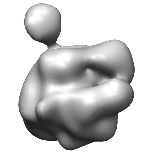

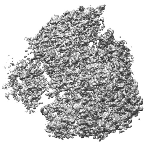
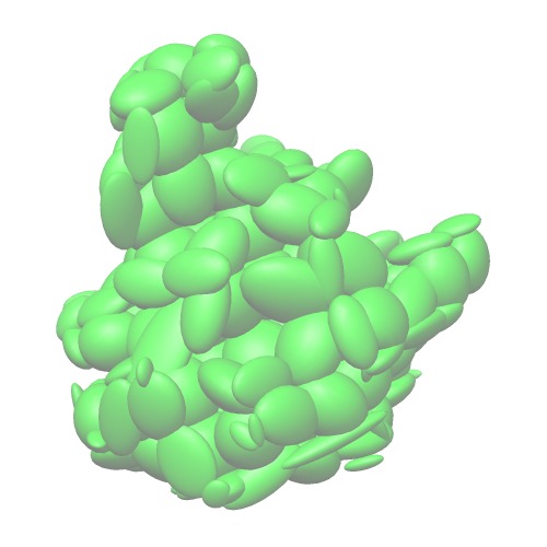
      original map (EMD-2190) with threshold 0.0666	Centers of GMM (emd_2190_ng10.gmm)	Wireframe of GMM isocontour surface (emd_2190_ng10_surface.wrl)	Ellipsoids of GMM (emd_2190_ng10_ellipsoid.wrl)

   2. Algorithm of fitting GMM with the density map

      The program gmconvert employs the EM (expectarion-maximization) algorithm for fittting GMM with the given density map.

      option -emalg	default or not	name	explanation
      WP		Weighted point-input GMM (WP-input GMM)	Each voxel is represented by the center point with weights of density
      G	default	Gaussian-input GMM (G-input GMM)	Each voxel is represented by the isotropic Gaussian function with variance = [grid_width]/12.
      D		Down-sampled Gaussian function (DSG)	Neighboring voxles are merged into one Gaussian functions. The option -dsfact is requried.
      DG		Down-sampled Gaussian-input GMM (DSG-input GMM)	Down-sampled Gaussian functions are used for the input of G-input GMM. The option -dsfact is requried.

      NOTE: The option -emalg P does not work for the density map.

      The convergence of the EM algorithm will be determined mainly by following two parameters.

      1. -nr: Number of repeat for EM [10000]
      2. -cv: Convergence threshold for dParam for the EM algorithm [0.001000]

      Especially, the option -nr strongly affects the computation time. The default value is -nr 10000. If less number is assigned, for example, -nr 1000, the program may finish before 1/10 computation time, although the final likelihood value may not be fully converged.

   3. For the map with large number of voxels

      It often requires large amount of time (more than hours) to convert the map with large number of voxels (such as 512³ voxles) into GMM. We recommend following two ways to the fast conversion of these large map.

      • Down-sampled Gaussian functions (DSG) :-emalg D

        The first way is employing the down-sampled Gaussian functions (DSG). This is merging neighboring voxels into one anisotropic Gaussian functions to generate GMM. An command example is as follows:

        gmconvert V2G -imap [map file] -ogmm [GMMfile] -zth [threshold] -emalg D -dsfact [down-sampling factor]
        

        Number of neighboring voxels can be controlled by the option -dsfact. [dsfact]³ voxels are merged into one Gaussian function. For example, if the option -dsfact 2 is assigned, 2 x 2 x 2 = 8 voxels are merged into one Gaussian function. In the case of -emalg D, the number of Gaussian functions of the GMM cannot be assigened by the option -ng, it depends on number of foreground voxels in the original map and the down-sampling factor -dsfact.

        Command examples using emd_6643 (512³ voxels) are shown as follows:

        gmconvert V2G -imap emd_6643.map -zth 0.018 -emalg D -dsfact 16 -ogmm emd_6643_D_df16.gmm
        

        gmconvert G2E -igmm emd_6643_D_df16.gmm -zth 0.018 -oewrl emd_6643_D_df16_ellipsoid.wrl -elcol W -elRGBT 0:0:0:0
        

        The genration of DSG is quite fast, because it does not require any iterative calulation. The DSG is suitable for generating a GMM with a large number of Gaussian functoins (such as > 1000) for a high-resolution density map.

      • Down-sampled Gaussian-input GMM (DSG-input GMM) :-emalg DG

        The second way is employing the DSG-input GMM. First, a down-sampled Gaussian functoins (DSG) is generated, then the Gaussian-input GMM alrogithm is applied to the genrated DSG. The DSG-input GMM is suitable for generating a GMM with a small number of Gaussian functoins (such as < 100). An command example is as follows:

        gmconvert V2G -imap [map file] -ogmm [GMMfile] -zth [threshold] -emalg DG -dsfact [down-sampling factor] -ng [Ngauss]
        

        Note that the option -ng is required for the case of the option DG. Command examples using emd_6643 (512³ voxels) are shown as follows:

        gmconvert V2G -imap emd_6643.map -zth 0.018 -emalg DG -dsfact 16 -ng 10 -ogmm emd_6643_DG_df16_ng10.gmm
        

        gmconvert G2E -igmm emd_6643_DG_df16_ng10.gmm -oewrl emd_6643_DG_df16_ng10_ellipsoid.wrl -elcol W -elRGBT 0:0:0:0
        

        Original map (EMD-6643) threshold density:0.018 Number of voxels 5123 Number of foreground voxels:2057291	Down-sampled Gaussian functions (DSG) by ellipsoidal representation. (emd_6643_D_df16_ellipsoid.wrl) Number of Gaussian functions: 2995	DSG-input GMM by ellipsoidal representation. (emd_6643_DG_df16_ng10_ellipsoid.wrl) Number of Gaussian functions: 10

      • Gaussian-input with down sampling (G) :-emalg G with -dsfact

        This is not our recommended way. The Gaussian-input GMM algorithm can also use the down-sampling using -dsfact. Different from the DG-input GMM (-emalg DG), the G-input GMM first converts the original map into a down sampled map with -dsfact, and regards the map as a set of "isotropic" Gaussian functions, not anistropic ones. An example is as follows:

        gmconvert V2G -imap emd_6643.map -zth 0.018 -emalg G -dsfact 16 -ng 10 -ogmm emd_6643_G_df16_ng10.gmm -omapds emd_6643_df16.map
        

        The input isotropic Gaussian functions can be seen as follows:

        gmconvert V2G -imap emd_6643_df16.map -zth 0.018 -emalg O -ogmm emd_6643_df16.gmm
        gmconvert G2E -igmm emd_6643_df16.gmm -oewrl emd_6643_df16_ellipsoid.wrl -elcol W -elRGBT 0:0:0:0
        

        As you see, the istropic Gaussian functions from the downsampled map less conserve the features of the original map than the anisotroic GMM. It does not conserve the covariance matrix of the original map.

        Isotropic Gaussian functions from down-sampled map(DSG) by ellipsoidal representation. (emd_6643_df16_ellipsoid.wrl) Number of Gaussian functions: 2995

   4. Other Options
      • -maxsize: allowed max voxel size of each axis. If over, downsample to isotropic gauss (-emalg G/WP) or anisotropic gauss (-emalg D). [-1]
      • -dsfact: downsampling factor (2,3,4,...) for -emalg G/W or -emalg D or -emalg DG. [1]
      • -vargrd : Variance type for grid points (for -emalg G or T). 'G':var = ww2var * grid_width * grid_width, 'R': var = (resolution/2.0)^2.[G]
      • -ww2var : Constant for variance = Const * grid_width*grid_width for emalg G. Default is 1/12 [0.083333].
      • -resogrd: Resolution for grid point (for -emalg G -vargrd R) [0.000000].
      • -resoblurgrd : Resolution of grid point for blurring the map. [0.000000].
      • -ogmm: Output Gaussian File (*.gmm) []
      • -ng: Number of Gaussian functions for GMM [1]
      • -emalg: type for EM algorithm. 'P'oint-input,'WP'eighted_point-input 'G'aussian-input (isotropic) 'O':1-to-1 atom/grid pnts : 'D':Down-sampled gaussians 'DG':Down-sampled gaussian-input GMM [G] : note: 'D' and 'DG' is only for map (V2G)
      • -I: Initialization of GMM. 'K'-means, 'R'andom 'O':one-to-one_atom/grid pnts [K]
      • -delzw: Delete Zero-weight gaussians from the GMM. ('T' or 'F') [T]
      • -delid: Delete identical gaussians in the GMM. ('T' or 'F') [T]
      • -nr: Number of repeat for EM [10000]
      • -nk: Number of repeat for K-means multi-start [1]
      • -cv: Convergence threshold for dParam for the EM algorithm [0.001000]
      • -olog: Output logfile []
      • -stdlog: output convergence log as stdout ('T' or 'F') [T]
      • -ogmminit: Output Initial Gaussian File before EM algorithm (*.gmm) []
      • -ogmmds: Output down-sampled Gaussian File for '-emalg D' or '-emalg DG'. (*.gmm) []
      • -omapds: Output down-sampled CCP4 density map file (*.map) []
      • -opost: Output PDB File for posterior probability []
      • -justcnt : just count input number_of_atom /map_size, and quit. ('T' or 'F') [F]
      • -rseed : random number seed(>=1) [1] -max_memory: maximum memory size in mega byte [1000]

5. Convert Atomic model into GMM
   1. Basic usage

      gmconvert A2G -ipdb [pdb file] -ng [number of Gaussians] -ogmm [output GMM file]
      

      For example, if you want to convert the pdb file 'pdb5c44.ent' into GMM with 10 Gaussian functions, a command is as follows:

      gmconvert A2G -ipdb pdb5c44.ent -ng 10 -ogmm 5c44_ng10.gmm
      

      The generated GMM can be visually checked by various formats. The simplest way is just open the generated "*.gmm" file as the PDB file by molecular graphics program. Then, the centers of Gaussian functions are shown.

      The isocontour surface model in VRML format (*.wrl) can be generated by the gmconvert by a following command:

      gmconvert G2S -igmm 5c44_ng10.gmm -owrl 5c44_ng10_surface.wrl
      

      The ellipsoid model in VRML format (*.wrl) can be generated by the gmconvert by a following command:

      gmconvert G2E -igmm 5c44_ng10.gmm -oewrl 5c44_ng10_ellipsoid.wrl
      

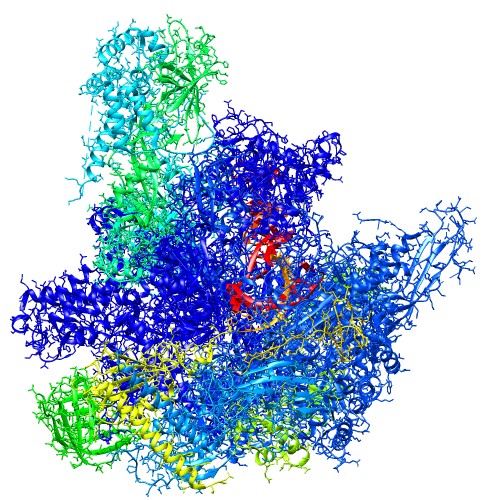
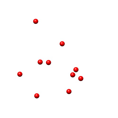
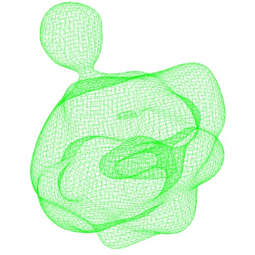
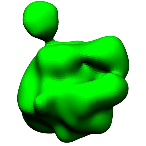
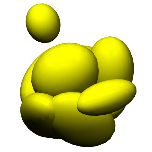
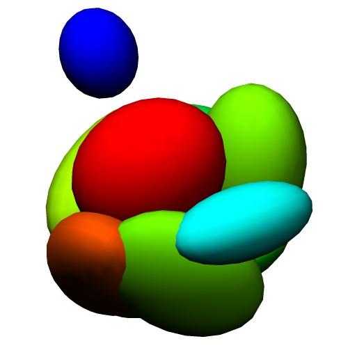
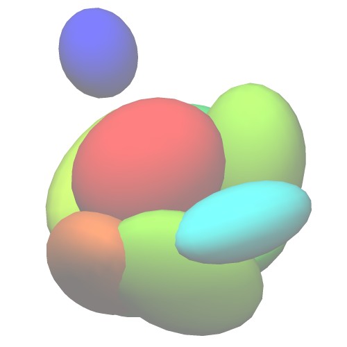
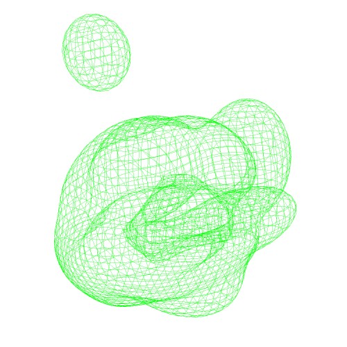
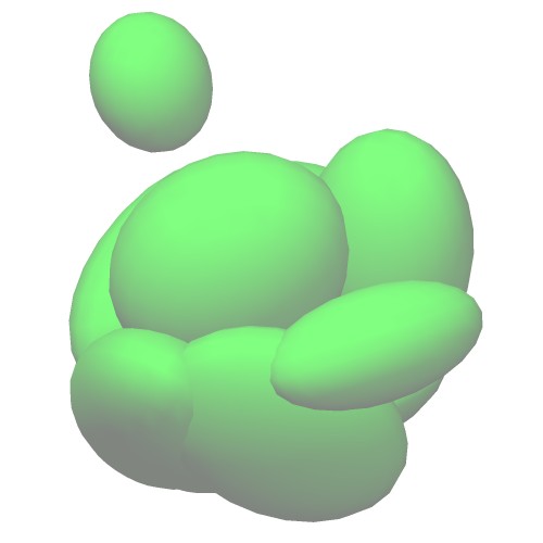
      Atomic Model (PDB ID:5c44)	Centers of GMM (5c44_ng10.gmm)	Wireframe of GMM isocontour surface (5c44_ng10_surface.wrl)	Ellipsoids of GMM (5c44_ng10_ellipsoid.wrl)

   2. Algorithm of fitting GMM with the atomic model

      The program gmconvert employs the EM (expectarion-maximization) algorithm for fittting GMM with the given atomic model.

      option	default or not	name	explanation
      -emalg P		Point-input GMM (P-input GMM)	Each atom is represented by the center points with equal weights
      -emalg WP		Weighted point-input GMM (WP-input GMM)	Each atom is represented by the center points with atomic weights
      -emalg G	default	Gaussian-input GMM (G-input GMM)	Each atom is represented by the isotropic Gaussian function with variance = [Rvdw]/5.

      NOTE: The options -emalg D and -emalg DG do not work for the atomic model.

   3. Options for input of the atomic model

      The program gmconvert can read both PDB file and mmCIF file:

      • -ipdb : Input PDB file for atomic model []
      • -icif : Input mmCIF file for atomic model []

      You can restrict atoms in the PDB file as follows:

      • -hetatm: Read HETATM ('T' or 'F') [F].
        The defaul is -hetatm F, it means the program only read "ATOM" line.
      • -ch: Chain ID. (or 'auth_asym_id' in mmCIF).
        The defaul is -ch -, it means the program reads all the chains in PDB file/mmCIF file.
      • -atmsel: Atom selection. 'A'll atom except hydrogen, 'R'esidue-based (only ' CA ' and ' P ') [A]
      • -model : 'S':read only single model (for NMR). 'M':read multiple models (for biological unit) [S]

      When a mmCIF file is input by the option -icif, you can assign assembly_id for biological units:

      • -assembly: assembly_id for mmCIF file (-icif) [].
        The assembly_id in mmCiF file (such as 1,2,3,PAU,XAU,..) can be assingned. The program performs symmetrc operations to asymmetric unit to generate XYZ coordinates of the assembly. If the option assembly_id is not assigned, the program use the asymmetric unit.

   4. Other options
      • -hetatm : Read HETATM ('T' or 'F') [F]
      • -ch : Chain ID. (or 'auth_asym_id' in mmCIF). [-]
      • -atmsel : Atom selection. 'A'll atom except hydrogen, 'R'esidue-based (only ' CA ' and ' P ') [A]
      • -maxatm : maximum allowed number of atoms for '-atmsel A'. If over '-maxatm', then change '-atmsel R'.[-1]
      • -atmrw : Model for radius and weight. 'A':atom model, 'R':residue model, 'M'ix of atom/residue. : 'U':uniform radius/weight,'C':decide from content. [C]
      • -radtype: radius type for '-atmrw A'. V:van der Waals radius, C:covalent radius [V]
      • -raduni : radius for uniform model for '-atmrw U'. [-1.000000]
      • -varatm : Variance type for atom. 'R':sig = reso/2, 'A': sig^2= rr2var*Rvdw^2 + (reso/2)^2 'L': Laskowski style. f(Rvdw) = f(0.0)/2 'H':Hard-sphere-type [A]
      • -rr2var : Constant for variance = Const * Rvdw*Rvdw for -emalg G -varatm A. Default is '1/5=0.2'. [0.200000].
      • -reso : Resolution for atom-to-vox (sigma = reso/2) [0.000000]
      • -orw : output radius-weight file []
      • -uniRgmm: use uniform-Radius GMM ('T' or 'F') [F]
      • -Runigmm: Radius for uniform-Radius GMM [3.800000]
      • -ccatm : Calculation Corr Coeff bwn Atoms and GMMs.(It takes times..) (T or F)[F]
      • -ogmmpc: Output Gaussian File with PC axis (*.gmm) []
      • -ompdb : Output PDB File with membership values (*.pdb) []
      • -impdb : Input PDB File with membership values (*.pdb) []
      • -ogmm : Output Gaussian File (*.gmm) []
      • -ng : Number of Gaussian functions for GMM [1]
      • -emalg: type for EM algorithm. 'P'oint-input,'WP'eighted_point-input 'G'aussian-input (isotropic) 'O':1-to-1 atom/grid pnts : 'D':Down-sampled gaussians 'DG':Down-sampled gaussian-input GMM [G] : note: 'D' and 'DG' is only for map (V2G)
      • -I : Initialization of GMM. 'K'-means, 'R'andom 'O':one-to-one_atom/grid pnts [K]
      • -delzw : Delete Zero-weight gaussians from the GMM. ('T' or 'F') [T]
      • -delid : Delete identical gaussians in the GMM. ('T' or 'F') [T]
      • -nr : Number of repeat for EM [10000]
      • -nk : Number of repeat for K-means multi-start [1]
      • -cv : Convergence threshold for dParam for the EM algorithm [0.001000]
      • -olog : Output logfile []
      • -stdlog: output convergence log as stdout ('T' or 'F') [T]
      • -ogmminit : Output Initial Gaussian File before EM algorithm (*.gmm) []
      • -ogmmds : Output down-sampled Gaussian File for '-emalg D' or '-emalg d'. (*.gmm) []
      • -omapds : Output down-sampled CCP4 density map file (*.map) []
      • -opost : Output PDB File for posterior probability []
      • -justcnt : just count input number_of_atom /map_size, and quit. ('T' or 'F') [F]
      • -rseed : random number seed(>=1) [1]
      • -max_memory : maximum memory size in mega byte [1000]

6. Convert into various models
   1. Convert density map or GMM into surface model [V2S|G2S]

      The program 'gmconvert' can generate the surface model of the contour surface of the density map or GMM. The basic usage is as follows:

      gmconvert V2S -imap [CCP4/MRC mapfile] -owrl [output surface VRML file]
      

      gmconvert G2S -igmm [GMM file] -owrl [output surface VRML file]
      

      In order to make a surface model, the standard marching cube algorithm is employed. When the input GMM file is assigned, the program converts the GMM into a density map, then the map is converted to a surface model using the marching cube algorithm.

      Instead of the VRML output file (-owrl), other ourput formats are available:

      • -opdb: Output PDB File (only wire model) (*.pdb) []
      • -owrl: Output VRML File (both surface and wire model) (*.wrl) []
      • -oobj: Output Object File (only surface model) (*.obj) []

      The appearance of surface VRML file can be controled by the option -mcSW.

      • -mcSW : model type. 'S'urface, 'W'ireframe [W]

      Following two commands are examples for surface and wireframe model:

      gmconvert V2S -imap emd_2190.map -mcth 0.0666 -mcSW S -owrl emd_2190_S.wrl 
      

      gmconvert V2S -imap emd_2190.map -mcth 0.0666 -mcSW W -owrl emd_2190_W.wrl 
      

      Wireframe model -mcSW W	Surface model -mcSW S

      The color and transparency of surface VRML file can be controled by the option -mcRGBT.

      • -mcRGBT : RGBT string (red:green:blue:transparency) [0:1:0:0]

      Following three commands are examples for 'Green, non-transparent', 'Green, half-transparent', and 'Blue, non-transparent'.

      gmconvert V2S -imap emd_2190.map -mcth 0.0666 -mcSW S -mcRGBT 1:0:0:0.5 -owrl emd_2190_RGBT_1_0_0_05.wrl  
      

      gmconvert V2S -imap emd_2190.map -mcth 0.0666 -mcSW S -mcRGBT 0:1:0:0.5 -owrl emd_2190_RGBT_0_1_0_05.wrl  
      

      gmconvert V2S -imap emd_2190.map -mcth 0.0666 -mcSW S -mcRGBT 0:0:1:0 -owrl emd_2190_RGBT_0_0_1_0.wrl  
      

      Green, non-transparent -mcRGBT 0:1:0:0	Green, half-transparent -mcRGBT 0:1:0:0.5	Blue, non-transparent -mcRGBT 0:0:1:0

      The other options for the marching cube algorithm is described as follows:

      • -mcsd : SD value for threshold density [3.000000]
      • -mcth : raw density value for threshold density [-1000.000000]
      • -mcnv : number for voxel for threshold density [-1]
      • -mcvo : volume (A^3) for threshold density [-1.000000]
      • -mcch : ChainID for output [X]
      • -mcofan : offset atom number [0]

      When the GMM is converted (the mode G2S), following addtional options are availble:

      • -gw : grid width (angstrom) [4.000000]
      • -omap : Output CCP4 density map file (*.map) []
      • -ovox : Output Voxel File []
      • -grdorg : Origin XYZ for grid (x:y:z) (optional) [::]
      • -grdN : Number of grid (x:y:z) (optional) [::]

   2. Convert GMM into ellipsoidal model[G2E]

      The GMM can be represented by ellipsoids. The ellipsoids is good to represent number of Gaussian function and shapes of each Gaussian function, although the boundary surface of GMM cannot be represented correctly. Basic usage is as follows:

      gmconvert G2E -igmm [input GMM file] -oewrl [output ellipsoidal VRML file]
      

      When a Gaussian function is converted into an ellipsoid, three axis of the ellipsoid correspond to the three principal axis (eigen vectors) of the covariance matrix of the Gaussian function. The three radii of the ellipsoid are determined so that they are proporitional to the root of the three eigen values of the covariance matrix.

      R1 = tau * sqrt(ev1),  R2 = tau * sqrt(ev2),  R3 = tau * sqrt(ev3) 
      

      where R1, R2, R3 are three radii of the elipsoid (R1>=R2>=R3), ev1, ev2, ev3 are three eigen values of the covariance matrix (ev1>=ev2>=ev3), and tau is the scaling parameter. The radius of gyration of the ellipsoid is:

      Rg_ellipsoid = (R1*R1 + R2*R2 + R3*R3)/5  = tau*tau * (ev1 + ev2 + ev3)/5 
      

      In contrast, the radius of gyration of the Gaussian function is:

      Rg_gaussian = ev1 * ev2 * ev2 
      

      If we assume two radius of gyration are the same (Rg_ellipsoid = Rg_gaussian), then tau = sqrt(5). The option -elscl R assigned the this scaling value (tau = sqrt(5)).
      
      • -elscl : type for scaling ellipsoid. 'C':use cover_ratio (-elcov), 'R': Rg-equivalent scale(scale=sqrt(5),elcov=0.828203)[C]
      The size of the ellipsoid is controlled by the option -elcov. The tau = sqrt(5) corresponds to -elcov 0.828203.
      • -elcov : cover ratio for ellipsoid scale (0..1). (larger value -> larger ellipsoid) [0.828203]
      If more larger ellipsoids are necessary, the larget value of the option -elcov has to be assigned.

      The color of the ellipsoids are assigned by various ways. If you want to color the ellipsoids in the same color, the color can be assigend by the option -elRGBT:

      • -elRGBT : RGBT string (red:green:blue:transparency) [0:1:0:0.5]
      If you want to color by weights of Gaussian functions, the option -elcol W has to be assigned. If you want to color by Gaussian function numbers, the option -elcol N has to be assigned.
      • -elcol : color type. 'W':by weights of gaussians. 'N':by gaussian number, 'P':by property otherwise:by '-elRGBT' option [X]
      For these cases, graduation of coloring is decided by the option elcolsch
      • -elcolsch: color scheme. 'BGR':blue->green->red, 'BWR':blue->white->red, 'KW':black->white 'pR':pale red ->red[BGR]
      Please note taht even for the option -elcol W and -elcol N, the transparency value is assigned the fourth column of the option -elRGBT.

      Other options are as follows:

      • -elshape : Shape of prototype ellipsoid. 'S':sphere, 'Y'cylinder, 'O':cone 'B':box [S]
      • -oeps : Output PostScript File for ellipses (*.ps) []

      Following three commands are examples for 'Yellow, non-transparent', 'Weight-color, non-transparent', and 'Weight-color, halft-transparent'.

       gmconvert G2E -igmm emd_2190_ng10.gmm  -elRGBT 1:1:0:0 -oewrl emd_2190_ng10_RGBT_1_1_0_0.wrl 
      

       gmconvert G2E -igmm emd_2190_ng10.gmm  -elcol W -elRGBT 0:0:0:0   -oewrl emd_2190_ng10_W.T0.wrl 
      

       gmconvert G2E -igmm emd_2190_ng10.gmm  -elcol W -elRGBT 0:0:0:0.5 -oewrl emd_2190_ng10_W_T05.wrl 
      

      Yellow, non-transparent -elRGBT 0:1:0:0	Weight-color, non-transparent -elcol W -elRGBT 0:0:0:0	Weight-color, transparent -elcol W -elRGBT 0:0:0:0.5

   3. Convert GMM into Density map[G2V]

      Basic usage is as follows:

        gmconvert G2V -igmm [GMM] -omap [CCP4/MRC map file] -gw [grid_width]
      

      Other options as follows:
      1. -omap : Output CCP4 density map file (*.map) []
      2. -ovox : Output Voxel File []
      3. -gw : grid width (angstrom) [4.000000]
      4. -grdorg : Origin XYZ for grid (x:y:z) (optional) [::]
      5. -grdN : Number of grid (x:y:z) (optional) [::]

   4. Convert Atomic model into Density map[A2V] Basic usage is as follows:

        gmconvert A2V -ipdb [PDBfile] -omap [CCP4/MRC map file] -reso [resolution]
      

      Options for input atomic models are the same as those of Convert Atomic model into GMM. Other options as follows:
      1. -omap : Output CCP4 density map file (*.map) []
      2. -ovox : Output Voxel File []
      3. -gw : grid width (angstrom) [4.000000]
      4. -reso : Resolution for atom-to-vox (sigma = reso/2) [0.000000]
      5. -grdorg : Origin XYZ for grid (x:y:z) (optional) [::]
      6. -grdN : Number of grid (x:y:z) (optional) [::]
      7. -occ : Output CorrCoeff file for the map of VdW atoms vs 3D density []

7. File formats For GMM
   1. *.gmm format

      An example of GMM (emd_2190.map, contourLevel:0.0666,Ngauss = 3) is shown as follows:

      HEADER 3D Gaussian Mixture Model
      REMARK COMMAND gmconvert V2G -imap emd_2190.map -zth 0.0666 -ng 3 -ogmm emd_2190_ng3.gmm
      REMARK START_DATE Sep 28,2017 20:47:2
      REMARK END_DATE   Sep 28,2017 20:47:10
      REMARK COMP_TIME_SEC  8.228681 8.228681e+00
      REMARK HOSTNAME   crambin
      REMARK FILENAME emd_2190_ng3.gmm
      REMARK NGAUSS 3
      REMARK RG 51.631184
      HETATM    1  GAU GAU G   1     208.396 181.147 205.548 0.366 0.366
      REMARK GAUSS     1 W 0.3662558729
      REMARK GAUSS     1 det  162993647.0996315479
      REMARK GAUSS     1 Cons 0.0000049733
      REMARK GAUSS     1 M 208.396429 181.147418 205.548323
      REMARK GAUSS     1 CovM  xx  984.2904266533 xy -108.8394668472 xz -488.6217524492
      REMARK GAUSS     1 CovM  yy  485.3174773738 yz  150.1245083477 zz  611.9590004288
      HETATM    2  GAU GAU G   2     190.647 154.028 162.044 0.312 0.312
      REMARK GAUSS     2 W 0.3124700981
      REMARK GAUSS     2 det  63293709.5044436157
      REMARK GAUSS     2 Cons 0.0000079809
      REMARK GAUSS     2 M 190.646737 154.028421 162.043696
      REMARK GAUSS     2 CovM  xx  797.2758963441 xy  -97.1173152835 xz   39.6808925721
      REMARK GAUSS     2 CovM  yy  343.5824098910 yz -189.6242080573 zz  344.2031563260
      HETATM    3  GAU GAU G   3     172.381 203.113 168.304 0.321 0.321
      REMARK GAUSS     3 W 0.3212740291
      REMARK GAUSS     3 det  64338148.2020744681
      REMARK GAUSS     3 Cons 0.0000079158
      REMARK GAUSS     3 M 172.381137 203.112891 168.303646
      REMARK GAUSS     3 CovM  xx  447.6521017988 xy  248.5348341885 xz   64.8458492268
      REMARK GAUSS     3 CovM  yy  434.6023355066 yz  -52.4706265936 zz  520.3255088737
      TER
      

      This is a pseudo-PDB format. If the molecular viewer program opens it as the PDB format, it reads only "HETATM" lines which describe centers of each Gaussian distribution function. However, the important information of this file is described in "REMARK" lines. Gaussian Mixture Model is the weighted sum of Gaussian Distribution Functions (GDFs). Its parameters are Ngauss(Number of GDFs) and Ngauss sets of { weight, center postiion(x,y,z), covariance matrix(3x3)}. The covariance matrix (CovM) is a 3x3 symmetric matrix, it requires only six parameters(xx,xy,xz,yy,yz,zz). These paramerers are described in a following format:

      REMARK NGAUSS [Number of GDFs for GMM]
      REMARK GAUSS   [GDFnumber] W [Weight for GDF] 
      REMARK GAUSS   [GDFnumber] M [Center position of GDF (x y z) ] 
      REMARK GAUSS   [GDFnumber] CovM  xx [xx of CovM]  xy  [xy of CovM] xz [xz of CovM] 
      REMARK GAUSS   [GDFnumber] CovM  yy [yy of CovM]  yz  [yz of CovM] zz [zz of CovM] 
      

   2. *.txt format

      The program gmconvert also can output a GMM in IMP (integrative modeling platform) format. An example of the same GMM (emd_2190.map, contourLevel:0.0666,Ngauss = 3) is shown as follows:

      #|num|weight|mean|covariance matrix|
      |0|0.366255872859|208.396429176811 181.147418229568 205.548322709826|984.290426653279 -108.839466847152 -488.621752449202 -108.839466847152 485.317477373770 150.124508347682 -488.621752449202 150.124508347682 611.959000428782|
      |1|0.312470098051|190.646737426874 154.028420880060 162.043695570500|797.275896344050 -97.117315283514 39.680892572120 -97.117315283514 343.582409890998 -189.624208057281 39.680892572120 -189.624208057281 344.203156325999|
      |2|0.321274029091|172.381136505073 203.112891158126 168.303645954442|447.652101798849 248.534834188489 64.845849226807 248.534834188489 434.602335506599 -52.470626593647 64.845849226807 -52.470626593647 520.325508873713|
      

      A GMM can be used as one of the representations of the molecules. A modeling example using GMM is available in the tutorial page of RNA polymerase II. A script for generating GMM is available as create_gmm.py.

8. References
   
   1. Kawabata, T. Multiple subunit fitting into a low-resolution density map of a macromolecular complex using a gaussian mixture model. Biophys J 2008 Nov 15;95(10):4643-58. [Publisher] [PubMed]
   2. Kawabata, T. Gaussian-input Gaussian mixture model for representing density maps and atomic models. J Struct Biol. Volume 203, Issue 1, July 2018, Pages 1-16 doi: 10.1016/j.jsb.2018.03.002. [Publisher] [PubMed]
   3. Pettersen, E.F., Goddard, T.D., Huang, C.C., Couch, G.S., Greenblatt, D.M., Meng, E.C., Ferrin, T.E.. UCSF Chimera--a visualization system for exploratory research and analysis. J Comput Chem. 2004 Oct;25(13):1605-12.